Bounded Static Analysis

Everything Everywhere All at Once

Table of Contents

What is Bounded Static Analysis?§1
1. In Theory§1.1
2. May and Must Analyses§1.2
Abstractions§2
Bounded Abstract Interpretation§3
Getting Started§4

In this topic we are going to make our first static analysis. It is based on abstract interpretation.

What is Bounded Static Analysis? §1

In bounded static analysis we want to talk about all the behaviors of the program up to some depth. There are no easy way to do this, because we have to handle a possible infinite set of traces, which by itself is hard to do.

The idea behind bounded static analysis is straight forward. Instead of selecting a single initial state and then applying the semantics on that until a trace has been made. This is what we did with dynamic analysis. We start with the set initial states and then apply the semantics to all states at once. Essentially, if dynamic analysis is depth first search, Static Analysis is breath first. While we have the downside of having to work with infinite sets of traces, we can be smart about it, and use abstractions to represent the set using a finite number of traces.

In Theory §1.1

The Bounded Static Analysis on a program $P$ can defined as the set of traces of depth $n$ : ${𝐁 𝐒 𝐀}_{P}^{n}$ . We can get this set using a many-stepping function $𝚜 𝚝 𝚎 𝚙$ . It takes a set of traces and steps them one step.

{𝚜 𝚝 𝚎 𝚙}_{P} (T) = {τ^{'} s | s \in Σ, τ^{'} \in T, δ_{P} ({τ^{'}}_{| τ^{'} |}, s)}

In the definition of $𝚜 𝚝 𝚎 𝚙$ , $δ$ is the transition relation defined by the single step semantics, and $τ^{'} s$ means appending $s$ to $τ^{'}$ . Since we are always talking about the same program $P$ we'll sometimes omit it.

Now, we can define the set of traces of up to length $n$ , as applying $𝚜 𝚝 𝚎 𝚙$ to the initial state, $n$ times, and taking the union of the results.

\begin{matrix} {𝚜 𝚝 𝚎 𝚙}_{P}^{0} & = I_{P} \\ {𝚜 𝚝 𝚎 𝚙}_{P}^{n} & = {𝚜 𝚝 𝚎 𝚙}_{P} ({𝚜 𝚝 𝚎 𝚙}_{P}^{n - 1}) \cup {𝚜 𝚝 𝚎 𝚙}_{P}^{n - 1} \end{matrix}

\begin{matrix} {𝐁 𝐒 𝐀}_{P}^{n} & = {𝚜 𝚝 𝚎 𝚙}_{P}^{n} \end{matrix}

Now, we can check for assertion errors down to depth $n$ . Let's call this ${𝐁 𝐀 𝐄}_{P}^{n}$ , by seeing if any trace ends in an assertion error:

{𝐁 𝐀 𝐄}_{P}^{n} \equiv \exists (τ s) \in {𝐁 𝐒 𝐀}_{P}^{n} \land s = err (‘𝚊𝚜𝚜𝚎𝚛𝚝𝚒𝚘𝚗 𝚎𝚛𝚛𝚘𝚛’)

May and Must Analyses §1.2

Sadly, it is infeasible, and sometimes impossible, to do computations over all traces at ones. Therefore, when designing an analysis, we either underestimate the set of traces. This is called a must analysis, or overestimate the set of traces which is called a may analysis. A must analysis is named like that, because we know what the program must do, and a may analysis is called that because we know what the program may do.

In a may analysis we overestimate every step, and in the must analysis we underestimate every step:

\begin{matrix} {𝚜 𝚝 𝚎 𝚙}_{𝗆 𝗎 𝗌 𝗍} (T) \subseteq 𝚜 𝚝 𝚎 𝚙 (T) \subseteq {𝚜 𝚝 𝚎 𝚙}_{𝗆 𝖺 𝗒} (T) \end{matrix}

Naturally, we'll see that

{𝚜 𝚝 𝚎 𝚙}_{𝗆 𝗎 𝗌 𝗍}^{n} \subseteq {𝚜 𝚝 𝚎 𝚙}^{n} \subseteq {𝚜 𝚝 𝚎 𝚙}_{𝗆 𝖺 𝗒}^{n}

The may analysis is great if we want to make sure that something newer happens. Essentially, if we want to warn about an assertion error may happen, we need a may analysis. If we want to grantee that an assertion error must happen on an run, then we need a must analysis:

\begin{matrix} {𝐁 𝐀 𝐄}_{𝗆 𝗎 𝗌 𝗍}^{n} ⟹ {𝐁 𝐀 𝐄}^{n} \\ \neg {𝐁 𝐀 𝐄}^{n} ⟸ \neg {𝐁 𝐀 𝐄}_{𝗆 𝖺 𝗒}^{n} \end{matrix}

However, it is unclear why allowing us to approximate the result will allow us to run the analyses at all. We need abstractions!

Abstractions §2

Instead of working with sets of traces, we have to work with finite structures instead. We call these abstractions.

The Sign Analysis §2.1

Before we go down into the theory, let's start with a concrete example.

Assume that we are working with all the possible integer values that an variable has at some point in the program. It would be much easier to simply keep track of whether the set contains positive, negative or zero values.

We can represent this as a set that only contain three elements ${+, -, 0}$ , exactly zero $(0)$ , larger than zero $(+)$ and smaller than zero $(-)$ . This set of size $3!$ , which is much easier to work with than the set of size $2^{32}!$ . In the following sections we are going to refer to this set as $𝐒 𝐢 𝐠 𝐧$ .

𝐒 𝐢 𝐠 𝐧 = {+, 0, -}

We call $𝐒 𝐢 𝐠 𝐧$ an abstraction, as we can covert the concrete domain of integers into the abstract domain of $𝐒 𝐢 𝐠 𝐧$ . We call this conversion the abstraction $α$ :

\begin{matrix} α ({1, 2, 3}) = & {+} \\ α ({0}) = & {0} \\ α ({- 1, 3}) = & {+, -} \\ α ({- 1, 0, 3}) = & {0, +, -} \end{matrix}

Make the Sign Abstraction

Implement the SignSet as an abstract set in the language of your choosing.

In Python, you can start with this:

from dataclasses import dataclass
from typing import TypeAlias, Literal

Sign : TypeAlias = Literal["+"] | Literal["-"] | Literal["0"]

@dataclass
class SignSet:
  signs : set[Sign]

However before we continue this set, we first have to ensure that a computation in abstract domain does not invalidate our over-approximation.

In the following sections we'll see that:

Our abstract domains can be ordered.
We can get the least over-approximation of two abstract sets called the join and the greatest under-approximation of two abstract sets called the meet.
Then, we have a formal definition of a correct over-approximating or under-approximating called a Galoi connection.
And finally, we'll cover monotone functions, which are function that preserves order.

Fasten your seatbelts it's going to be a bumby night!

Partially Ordered Sets (Posets) §2.2

Partially ordered set - Wikipedia

A partially ordered set or poset is a tuple $(L, ⊑)$ set of elements $L$ and an ordering $⊑$ , that uphold:

\begin{matrix} reflexive & \forall a . a ⊑ a \\ antisymetric & \forall a . a ⊑ b \land b ⊑ a ⟹ a = b \\ transitive & \forall a . a ⊑ b \land b ⊑ c ⟹ a ⊑ c \end{matrix}

Common partially ordered sets are the integers $(ℤ, \leq)$ (also in the other direction $(ℤ, \geq)$ ), the booleans $({𝚝 𝚝, 𝚏 𝚏}, \Rightarrow)$ , and the set of ${𝐒 𝐢 𝐠 𝐧}^{'} s$ $(2^{𝐒 𝐢 𝐠 𝐧}, \subseteq)$ .

Check the rules

Think about if the rules apply to the posets above.

Make Sign a partially ordered set

Make your $𝐒 𝐢 𝐠 𝐧$ abstraction into a partially ordered set by implementing $⊑$ (<=) in the language of your choice.

Lattices §2.3

A lattice is partially ordered sets $(L, ⊑)$ , with two extra operators $⊔$ and $⊓$ . $⊔$ is the least upper bound $a ⊔ b$ , meaning that

\forall c . a ⊑ c \land b ⊑ c ⟹ a ⊔ b ⊑ c .

The dual is true for $⊓$ that is the greatest lower bound

\forall c . c ⊑ a \land c ⊑ b ⟹ c ⊑ a ⊓ b .

Furthermore, this implies that there exist a least bound $⊥ = ⨅ L$ and a greatest bound $⊤ = ⨆ L$ , from which we have the following identities: $⊤ ⊓ a = a = a ⊔ ⊥$ , and $⊤ ⊔ a = ⊤$ and $a ⊓ ⊥ = ⊥$ .

Hasse diagrams. §2.3.1

Hasse diagram - Wikipedia

A Hasse diagram over the poset $(2^{𝐒 𝐢 𝐠 𝐧}, \subseteq)$ . By I, KSmrq, CC BY-SA 3.0 (with edits)

The reason why they are called latices is that they can be drawn using Hasse digrams which gives these nice structures, which looks like a wooden lattice.

Here we only draw the imitate next elements in the order. So while ${+} \subseteq {+, 0, -}$ we do not draw that edge because ${+, 0}$ and ${+, -}$ are in the way.

Rate your favourite animals

Create a Hasse diagram over your favorite animals, The order is $(𝐀𝐧𝐢𝐦, ‘𝚒𝚜 𝚠𝚘𝚛𝚜𝚎 𝚝𝚑𝚊𝚗’)$ . Where

𝐀𝐧𝐢𝐦 = {Cat, Dog, Ant, Worm, Spider, Horse, Rabbit}

While objectively $(Cat ‘𝚒𝚜 𝚠𝚘𝚛𝚜𝚎 𝚝𝚑𝚊𝚗’ Dog)$ some of the other animals like $Ant$ and $Worm$ are no worse than each other.

Is your order a lattice: Does every pair of animals have meet and a join?

Back to the Sign Abstraction §2.3.2

In our Sign abstraction, we use set inclusion as our order $⊑_{𝐒 𝐢 𝐠 𝐧} = \subseteq$ and use the intersection and union of the underlying set as the meet ( $⊓$ ) and join ( $⊔$ ) of our lattice. $⊥ = \emptyset$ and $⊤ = {+, -, 0}$ .

Make the Sign a lattice

To make your $𝐒 𝐢 𝐠 𝐧$ abstraction into a lattice, you need to also implement the meet $⊓$ and join $⊔$ operators.

In Python, you can implement __and__ and __or__ to get the meet operator a & b, and the join operator a | b.

Galois Connection §2.4

Galois connection - Wikipedia

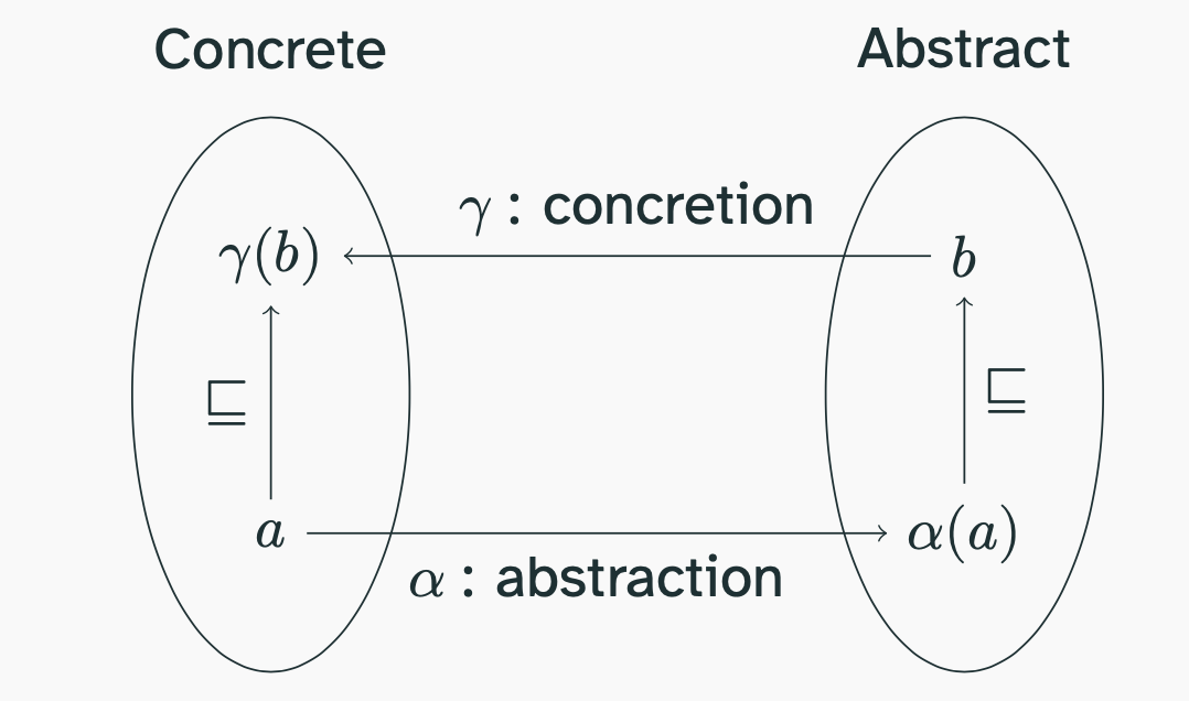
(A Galois Connection is a connection between two ordered sets, with a concretion $γ$ and an abstraction $α$ function.)

A Galois connection is a relationship between two ordered sets $(C, ⊑_{C})$ and $(A, ⊑_{A})$ , where we can abstract information from the concrete domain into the abstract $α : C \to A$ while preserving the order if going back $γ : A \to C$ . $α$ explains how to abstract a value, and $γ$ explains what the abstraction means.

Because the abstraction might be lossy it is not the case that if we abstract a value we get back the same concrete value $γ (α (c)) \neq c$ . Instead a Galois connection satisfies the following rule:

\forall c \in C, a \in A . c ⊑_{C} γ (a) \Leftrightarrow α (c) ⊑_{A} a

It states, that if we have a concrete value $c$ , and abstract it $α (c)$ , then any value larger than this abstraction $a$ will concertize to a value $γ (a)$ that is larger than the original value. At first this might not seem useful, but if we satisfy this rule we get the following laws for free:

\begin{matrix} c ⊑_{C} γ (α (c)) & – if we abstract we only increase in size \\ α (γ (a)) ⊑_{A} a & – if we concertize we only decrease in size \\ α (γ (α (c))) = α (c) & – we don’t keep loosing information \\ γ (α (γ (a))) = γ (a) & – in both directions \\ γ (a_{1} ⊔_{A} a_{2}) = γ (a_{1}) ⊔_{C} γ (a_{2}) & – γ preserves joins. \\ α (c_{1} ⊓_{C} c_{2}) = α (c_{1}) ⊓_{A} α (c_{2}) & – α preserves meets. \end{matrix}

The two first rules gives us confidence that whatever abstraction we choose only lose information never create it. And the second two rules gives us confidence that we don't keep losing that information.

Adjunctions and testing

Galoi connections is actually a concrete example on a mathematical construct called adjunction. Adjunctions are one of the most useful and unappreciated mathematical structures in computer science. One example is testing technique for testing data readers.

While in most cases we would expect, anything we pretty print to be parsable to the same value. That is not always the case as line numbers might differ or some data are lost in the translation. It should, however, always hold that

# Most of the time
parse(pretty(a)) == a 

# Always
pretty(parse(pretty(a))) == pretty(a)

# Bonus for all strings s:
parse(pretty(parse(s))) == parse(s)

Back to the Sign Analysis §2.4.1

We can see that there exist a Galoi connection between our concrete integer domain and our abstract sign domain $(2^{ℤ}, \subseteq) \leftrightarrow_{γ}^{α} (𝐒 𝐢 𝐠 𝐧, ⊑_{𝐒 𝐢 𝐠 𝐧})$ . Where the abstraction $α$ and concretion $γ$ are defined like this:

\begin{matrix} α (N) & = {+ | n \in N, n < 0} \\ \cup {- | n \in N, n > 0} \\ \cup {0 | n \in N, n = 0} \\ γ (S) & = {n | n \in ℤ, n < 0, + \in S} \\ \cup {n | n \in ℤ, n > 0, - \in S} \\ \cup {0 | 0 \in S} \end{matrix}

We can also see that we satisfy the rules, let's pick a concrete value ${0, 1}$ . If we convert that to an abstract value we get: $α ({0, 1}) = {0, +}$ .

Since $α ({0, 1}) ⊑ {0, +} ⊑ {0, +, -}$ , and since $γ ({0, +}) = ℤ^{0, +}$ and $γ ({0, +, -}) = ℤ^{0, +, -}$ , then we get that ${0, 1} \subseteq ℤ^{0, +} \subseteq ℤ$ .

Build the Sign abstraction

You need an abstract function, which takes a set and turns it into your abstract domain.

@classmethod
def abstract(cls, items : set[int]): 
  signset = set()
  if 0 in items:
    signset.add("0")
  ...
  return cls(signset)

Then because we are using possible infinite sets, instead of generating that set, we can just implement the contains method:

def __contains__(self, member : int): 
  if (member == 0 and "0" in self.signs): 
      return True
  ...

You can use the Galoi rules to test your abstraction:

\forall X \subset 2^{ℤ} : X \subseteq γ (α (X))

If you are using python you fuzz test this property using hypothesis.

from hypothesis import given
from hypothesis.strategies import integers, sets

@given(sets(integers()))
def test_valid_abstraction(xs):
  s = SignSet.abstract(xs) 
  assert all(x in s for x in xs)

Abstract Operations §2.5

Finally, we have reached the fun part. We can now define operations in the abstract domain that mimic the operations in the concrete.

Because our concrete domain is the set of integers, we can define $+_{2^{i 32}}$ , as the operation over the product:

\begin{matrix} A +_{2^{i 32}} B & = {a + b | a \in A, b \in B} \\ {1, 3} +_{2^{i 32}} {0, 10} & = {1, 3, 11, 13} \end{matrix}

Now we can also define the plus abstract domain:

\begin{matrix} {+} +_{𝐒 𝐢 𝐠 𝐧} {+} = & {+} & {+} +_{𝐒 𝐢 𝐠 𝐧} {-} = {-, +, 0} \\ {+} +_{𝐒 𝐢 𝐠 𝐧} {0} = & {+} & {0} +_{𝐒 𝐢 𝐠 𝐧} {+} = {+} \\ {0} +_{𝐒 𝐢 𝐠 𝐧} {-} = & {-} & {0} +_{𝐒 𝐢 𝐠 𝐧} {0} = {0} \\ {-} +_{𝐒 𝐢 𝐠 𝐧} {+} = & {-, +, 0} & {-} +_{𝐒 𝐢 𝐠 𝐧} {-} = {-} \\ {-} +_{𝐒 𝐢 𝐠 𝐧} {0} = & {-} & \dots \end{matrix}

And many more.

But, how do we know if we have implemented our abstract operation correctly? Since we want to over-approximate our operations, we know that computing in our abstract domain should newer under-approximate:

A +_{2^{i 32}} B \subseteq γ (α (A) +_{𝐒 𝐢 𝐠 𝐧} α (B))

The above equation requires us to create huge sets of values. Instead we can use our Galoi connection to rewrite the equation to see that, we only have to show the following:

α (A +_{2^{i 32}} B) \subseteq α (A) +_{𝐒 𝐢 𝐠 𝐧} α (B)

Essentially, abstracting the result of an operation, should be smaller than abstracting and doing the operation in the abstract domain.

Implement Abstract Arithmetic

Implement arithmetic for your sign abstraction.

In Python, you can build an Arithmetic class that can handle all the abstract arithmetics. Also if you use hypothesis, you can test that we have done the conversion correctly by, testing the following:

@given(sets(integers()), sets(integers()))
def test_sign_adds(xs, ys):
  assert (
    SignSet.abstract({x + y for x in xs for y in ys}) 
      <= SignSet.abstract(xs) + SignSet.abstract(ys)
    )

For cases, where we compare like le, we might want to return set of booleans instead.

@given(sets(integers()), sets(integers()))
def test_sign_adds(xs, ys):
    assert (
      {x <= y for x in xs for y in ys} 
      <= arithmetic.compare("le", SignSet.abstract(xs), SignSet.abstract(ys))
      )

In practice, Galoi connections allows us to map our infinite domain of may or must analyses into a more manageable abstract domain, while giving us guarantees that we are still correctly over- or under-estimating.

Let's assume we are building a may analysis. Since we want to over approximate our $𝚜 𝚝 𝚎 𝚙$ function, we therefore introduce an abstract domain $(A, ⊑_{A})$ that has an abstract stepping function ${𝚜 𝚝 𝚎 𝚙}_{A}$ . We assume the galoi connection $(2^{𝐓 𝐫 𝐚 𝐜 𝐞}, \subseteq) \leftrightarrow_{γ}^{α} (A, ⊑_{A})$ . We can use this new abstract stepping function to define an bounded static analysis of depth $n$ : ${𝐁 𝐒 𝐀}_{A}^{n} = {𝚜 𝚝 𝚎 𝚙}_{A}^{n}$ . We define ${𝚜 𝚝 𝚎 𝚙}^{n}$ recursively:

\begin{matrix} {𝚜 𝚝 𝚎 𝚙}_{A}^{0} & = α (I_{P}) \\ {𝚜 𝚝 𝚎 𝚙}_{A}^{n} & = {𝚜 𝚝 𝚎 𝚙}_{A} ({𝚜 𝚝 𝚎 𝚙}_{A}^{n - 1}) ⊔_{A} {𝚜 𝚝 𝚎 𝚙}_{A}^{n - 1} \end{matrix}

We can prove by induction over $n$ that stepping in the abstract domain is in fact a may analysis ${𝐁 𝐒 𝐀}^{n} \subseteq γ ({𝐁 𝐒 𝐀}_{A}^{n})$ , given that

𝚜 𝚝 𝚎 𝚙 (T) \cup T \subseteq γ ({𝚜 𝚝 𝚎 𝚙}_{A} (α (T)) ⊔_{A} α (T)) .

Show that ${𝐁 𝐒 𝐀}_{A}^{n}$ a may analysis

Using induction over $n$ , show that the following is true: $𝚜 𝚝 𝚎 𝚙 (T) \cup T \subseteq γ ({𝚜 𝚝 𝚎 𝚙}_{A} (α (T)) ⊔_{A} α (T)) ⟹ {𝐁 𝐒 𝐀}^{n} \subseteq γ ({𝐁 𝐒 𝐀}_{A}^{n})$

We can also show that $𝚜 𝚝 𝚎 𝚙 (T) \subseteq γ ({𝚜 𝚝 𝚎 𝚙}_{A} (α (T))$ is a stronger statement, and is sufficient to prove the above, by seeing that $𝚜 𝚝 𝚎 𝚙 (T) \cup T \subseteq γ ({𝚜 𝚝 𝚎 𝚙}_{A} (α (T)) ⊔_{A} α (T)) .$ From $T \subseteq γ (α (T))$ , And using that gamma preserves meets we get $𝚜 𝚝 𝚎 𝚙 (T) \cup T \subseteq γ ({𝚜 𝚝 𝚎 𝚙}_{A} (α (T)) \cup γ (α (T)) = γ ({𝚜 𝚝 𝚎 𝚙}_{A} (α (T) ⊔_{A} α (T))$

Finally, as it is very hard to talk about the concrete domain, as it is infinite, we can use the galoi connection again to see that we only have to show:

α (𝚜 𝚝 𝚎 𝚙 (T)) ⊑_{A} {𝚜 𝚝 𝚎 𝚙}_{A} (α (T))

The State Abstraction §3.1

The first, and most useful abstraction, is the state abstraction. Here we throw away everything from the trace except the final state of the trace:

(2^{𝐓 𝐫 𝐚 𝐜 𝐞}, \subseteq) \leftrightarrow_{γ}^{α} (2^{𝐒 𝐭 𝐚 𝐭 𝐞}, \subseteq)

We can define the abstraction as the set of end states of the traces and the concretion as the set of traces that end in one of the states.

\begin{matrix} α (T) = {τ_{| τ |} | τ \in T} \\ γ (S) = {τ | s \in S, τ \in 𝐓 𝐫 𝐚 𝐜 𝐞, τ_{| τ |} = s} \end{matrix}

This is a useful abstraction for us, because we do not need to know where the trace came from to figure out if an assertion error exist in the program, only that a trace ends in an assertion error.

We can now define ${𝚜 𝚝 𝚎 𝚙}_{𝐒 𝐭 𝐚 𝐭 𝐞}$ as only stepping the final state of each trace:

{𝚜 𝚝 𝚎 𝚙}_{𝐒 𝐭 𝐚 𝐭 𝐞} (S) = {s^{'} | s \in S, δ (s, s^{'})}

Check that ${𝚜 𝚝 𝚎 𝚙}_{𝐒 𝐭 𝐚 𝐭 𝐞}$ is an abstract operation of $𝚜 𝚝 𝚎 𝚙$

α (𝚜 𝚝 𝚎 𝚙 (T)) \subseteq {𝚜 𝚝 𝚎 𝚙}_{𝐒 𝐭 𝐚 𝐭 𝐞} (α (T))

Now let ${𝐁 𝐒 𝐀}_{𝐒 𝐭 𝐚 𝐭 𝐞}^{n} = {𝚜 𝚝 𝚎 𝚙}_{𝐒 𝐭 𝐚 𝐭 𝐞}^{n} (α (I_{P}))$ . It is now clear by induction on $n$ that ${𝐁 𝐒 𝐀}^{n} \subseteq γ ({𝐁 𝐒 𝐀}_{𝐒 𝐭 𝐚 𝐭 𝐞}^{n})$ . So if there exist an assertion error within $n$ steps, then there exist a trace $τ \in {𝐁 𝐒 𝐀}^{n}$ st. $τ_{| τ |} = err (‘𝚊𝚜𝚜𝚎𝚛𝚝𝚒𝚘𝚗 𝚎𝚛𝚛𝚘𝚛’)$ and $| τ | \leq n$ .

From our Galoi connection we can see that

\begin{matrix} {τ err (‘𝚊𝚜𝚜𝚎𝚛𝚝𝚒𝚘𝚗 𝚎𝚛𝚛𝚘𝚛’)} & \subseteq {𝐁 𝐒 𝐀}^{n} \subseteq γ ({𝐁 𝐒 𝐀}_{𝐒 𝐭 𝐚 𝐭 𝐞}^{n}) \\ ⟹ & α ({τ err (‘𝚊𝚜𝚜𝚎𝚛𝚝𝚒𝚘𝚗 𝚎𝚛𝚛𝚘𝚛’)}) \\ \subseteq {err (‘𝚊𝚜𝚜𝚎𝚛𝚝𝚒𝚘𝚗 𝚎𝚛𝚛𝚘𝚛’)} \\ \subseteq {𝐁 𝐒 𝐀}_{𝐒 𝐭 𝐚 𝐭 𝐞}^{n} \end{matrix}

Which means that if $err (‘𝚊𝚜𝚜𝚎𝚛𝚝𝚒𝚘𝚗 𝚎𝚛𝚛𝚘𝚛’) \notin {𝐁 𝐒 𝐀}_{𝐒 𝐭 𝐚 𝐭 𝐞}^{n}$ , then ${τ err (‘𝚊𝚜𝚜𝚎𝚛𝚝𝚒𝚘𝚗 𝚎𝚛𝚛𝚘𝚛’)} ⊈ {𝐁 𝐒 𝐀}^{n}$ . Which is exactly the grantee we are looking for in a may analysis.

The Per-Instruction Abstraction §3.2

In our next abstraction, we want to take advantage of that execute the same instruction in states with the same program counter.

Let's focus on a JVM without a method stack, which means that every state is $⟨ σ, λ, ι ⟩$ . We'll get back to talk about how to handle the method stack in later sections. We can abstract this by collecting the states per $ι$ . Let $𝐏 𝐜 = ι \to 2^{𝐒 𝐭 𝐚 𝐭 𝐞}$ be a mapping from program counters to sets of states. $𝐏 𝐜$ is a lattice with partial order $⊑_{𝐏 𝐜}$ were one mapping is less than another if all states are smaller than the other and $⊔_{𝐏 𝐜}$ is pointwise $\cup$ of states.

(2^{𝐒 𝐭 𝐚 𝐭 𝐞}, \subseteq) \leftrightarrow_{γ}^{α} (𝐏 𝐜, ⊑_{𝐏 𝐜})

Convince yourself this is a Galoi connection

Now we can write a stepping function that can step all states with the same instruction at once ${𝚜 𝚝 𝚎 𝚙}_{ι}$ , and then merge the result into the other states.

{𝚜 𝚝 𝚎 𝚙}_{𝐏 𝐜} (C) = ⨆_{𝐏 𝐜} {ι^{'} \mapsto {⟨ σ^{'}, λ^{'}, ι^{'} ⟩} | \begin{matrix} (ι \mapsto S) \in C, S^{'} = {𝚜 𝚝 𝚎 𝚙}_{ι} (S), \\ ⟨ σ^{'}, λ^{'}, ι^{'} ⟩ \in S^{'} \end{matrix}}

The Per-Variable Abstraction §3.3

We are now faced with our first hard choice.

We would love to use the Sign abstraction, that we build in the previous section, one way of doing that is compressing the state, so that instead of having a set of states, we distribute the content of the locals and stack. So instead of having a set of states, we have a pair of abstract locals and abstract stack. The abstract locals is not a mapping from naturals to a powerset of possible values, and the abstract stack is stack of possible values:

𝐏 𝐯 = ι \to (ℕ \mapsto (2^{𝐕_{σ}})) \times (2^{𝐕_{σ}}) * \cup {ok, err (‘.’)}

Since the stack and the locals are typed at each instruction, these are actually sets of integers, which we know how to abstract using the sign abstraction. Furthermore $𝐏 𝐯$ is also a partially ordered set, by point wise comparing the set of variables, and a lattice by point-wise joining and meeting the sets of variables. We can also see that $𝐏 𝐜 \leftrightarrow_{γ}^{α} 𝐏 𝐯)$ is a galoi connection.

The problem with this abstraction, and the reason this choice is hard, is that is the first that severely over-approximates our problem. More about this next time.

Define the Abstract State

Define the Abstract (per variable) Frame in your program analysis, remember to define the ordering as well as the meet and join operations. It might be useful to define three pseudo elements Bot, is an element that joins with all others, Err represent the error state and Ok represent the Ok state.

In Python, we could define an abstract frame like so:

@dataclass
class PerVarFrame[AV]:
  locals: dict[int, V]
  stack: Stack[AV]

Remember to define the abstract, __le__, __and__, and __or__ methods.

Variable Abstractions §3.4

Finally, we are at a point where we can use our Sign Abstraction, by using it to abstract the sets of variables.

𝐏 𝐯 [A] = ι \to (ℕ \mapsto A) \times A * \cup {ok, err (‘.’)}

If we can see $A$ is an abstraction of $2^{𝐕_{σ}}$ , then we also get a Galoi connection from $𝐏 𝐯$ to $P v [A]$ .

(2^{𝐕_{σ}}, \subseteq) \leftrightarrow_{γ}^{α} (A, ⊑_{A}) ⟹ (𝐏 𝐯, ⊑_{𝐏 𝐯}) \leftrightarrow_{γ}^{α} (𝐏 𝐯 [A], ⊑_{𝐏 𝐯 [A]})

Specifically, we get:

(𝐏 𝐯, ⊑_{𝐏 𝐯}) \leftrightarrow_{γ}^{α} (𝐏 𝐯 [𝐒 𝐢 𝐠 𝐧], ⊑_{𝐏 𝐯 [𝐒 𝐢 𝐠 𝐧]})

Experiment with different Abstractions

You have been introduced to the Sign Abstraction, but next time we'll look at more different abstractions. If you have time, try to come up with your own.

Abstractions All The Way Down. §3.5

One great thing about Galoi connections is that they compose. This mean we can create one long chain:

\begin{matrix} (2^{𝐓 𝐫 𝐚 𝐜 𝐞}, \subseteq) & \leftrightarrow_{γ}^{α} (2^{𝐒 𝐭 𝐚 𝐭 𝐞}, \subseteq) \\ \leftrightarrow_{γ}^{α} (𝐏 𝐜, ⊑_{𝐏 𝐜}) \\ \leftrightarrow_{γ}^{α} (𝐏 𝐯, ⊑_{𝐏 𝐯}) \\ \leftrightarrow_{γ}^{α} (𝐏 𝐯 [𝐒 𝐢 𝐠 𝐧], ⊑_{𝐏 𝐯 [𝐒 𝐢 𝐠 𝐧]}) \end{matrix}

Getting Started §4

To get started with the building your first static analysis, first refactor your interpreter to handle a more abstract state.

First, don't try to do everything at once! Start with a single frame.

Then, we need to realize that we can no longer return just one state. Eg., in the case where we are handling ifz we might need to return two states one where we jump and one where we don't.

def step(state : AState) -> Iterable[AState | str]
  ...

Secondly, do all the steps at once:

def many_step(state : dict[Pc, AState | str]) 
  -> dict[Pc, AState | str]:
  new_state = dict(state)
  for k, v in state.items():
      for s in step(v):
        new_state[s.pc] |= s
  return new_state

Until next time!

Until next time, write the best analysis you can and upload the results to Autolab, and ponder the following:

Why should we use abstractions when analysing code?
What is the advantage of Galoi connections?
Which cases are the Sign abstraction not able to catch?
At which cases do your static analysis outperform your dynamic?

Bibliography

Cousot, Patrick; Cousot, Radhia (1977). Abstract interpretation. doi:10.1145/512950.512973 link
Cousot, Patrick; Cousot, Radhia (1979). Systematic design of program analysis frameworks. doi:pdf/10.1145/567752.567778 link
Nielson, Hanne Riis; Nielson, Flemming (2007). Semantics with Applications.