Semantics

Let's give meaning to it all.

Christian Gram Kalhauge

The goal of this chapter is to ask and answer the following questions:

What was the hardest instruction to implement?
How big share of the cases were you able interpret?
Which part of the documentation was lacking?

1. What are Semantics?

isbn:978-1-84628-691-9

Today we are going to talk about semantics. Program semantics is about assigning meaning to programs. When we can talk about what program mean, it is easier to explain what they do.

We are going to discuss some different approaches to write down the semantics of a program. They all essentially turn programs syntax into mathematical logic.

1.1. Preface: Natural Deduction

Natural deduction, Wikipedia.

If you are unfamiliar with Natural Deduction and Gentzen-style proofs, please refer to the wikipediea page on the topic. The sort story is that we refer to logical rules like this:

\frac{{𝑝 𝑟 𝑒 𝑚 𝑖 𝑠}_{1} \dots {𝑝 𝑟 𝑒 𝑚 𝑖 𝑠}_{n}}{𝑐 𝑜 𝑛 𝑐 𝑙 𝑢 𝑠 𝑖 𝑜 𝑛} (n a m e)

Which means that ${𝑝 𝑟 𝑒 𝑚 𝑖 𝑠}_{1} \land \dots \land {𝑝 𝑟 𝑒 𝑚 𝑖 𝑠}_{n}$ implies $𝑐 𝑜 𝑛 𝑐 𝑙 𝑢 𝑠 𝑖 𝑜 𝑛$ .

If we want multiple ways of reaching the conclusion, we can make more rules. For example, conjunction $A \land B$ only requires one rule, both $A$ and $B$ has to be true but disjunction $A \lor B$ has two rules: either $A$ has to be true or $B$ has to be true.

\frac{A B}{A \land B} (\land) \frac{A}{A \lor B} (\lor_{L}) \frac{B}{A \lor B} (\lor_{R})

1.2. Axiomatic Semantics, Flowcharts, and Hoare Triplets

Hoare logic, Wikipedia.
homepage.divms.uiowa.edu/~slonnegr/plf/Book/Chapter11.pdf
doi:10.1007/978-94-011-1793-7_4

The first approach to assigning meaning to programs was Axiomatic Semantics. Here the meaning of the program is described by assigning precondition and postconditions to all statements in a program.

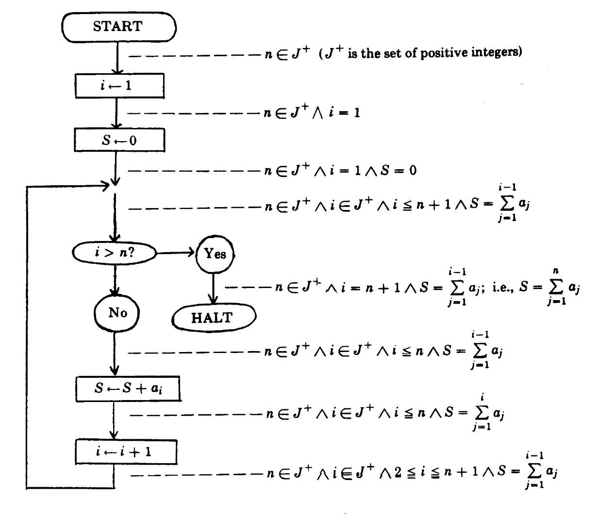
**Figure:** The flowchart from the original paper on semantics Assigning Meaning to Programs by Robert W. Floyd. The program computes the sum of an array.

In this world we can describe the semantics of a program by denoting three parts, the precondition $P$ , the program $C$ , and the postcondition $Q$ , this is also called Hoare triplets.

{P} C {Q}

These mean that if the world satisfies $P$ before executing $C$ then the world will satisfy $Q$ after.

The great thing about this approach is that we can compose the proofs of correctness of parts of the program into a proof of total correctness. Assume the program $C_{1}; C_{2}$ , where $C_{2}$ is executed after $C_{1}$ . Then we can describe the correctness of $C_{1}; C_{2}$ , like so:

\frac{{P_{1}} C_{1} {Q_{1}} {P_{2}} C_{2} {Q_{2}} Q_{1} \Rightarrow P_{2}}{{P} C_{1}; C_{2} {Q}}

If you are unfamiliar with the syntax above, it is natural deduction see the section on natural deduction. Essentially it means that given ${P_{1}} C_{1} {Q_{1}}$ , and ${P_{2}} C_{2} {Q_{2}}$ , and that the postcondition of $C_{1}$ implies the precondition of $C_{2}$ $(Q_{1} \Rightarrow P_{2})$ , are all true, we can also prove that ${P} C_{1}; C_{2} {Q}$ .

This approach is every effective at describing the meaning of specific programs. This means that it is very good for doing program verification, but is not used often for program analysis in general.

1.3. Denotational Semantics

Another approach for writing down the semantics of the program is Denotational Semantics. The idea behind denotational semantics is to map the semantics of the program we want to analyse to a program to something we know well. This can either be another programming language or math.

Consider a very simple expressional language called $𝔼 𝕏$ , which has addition, variables $x$ and natural numbers $n$ :

e \in 𝔼 𝕏 := e_{1} + e_{2} | x | n

If want to give meaning to the $𝔼 𝕏$ program x + 5, then we can define a map from expressions to a function from a store to integers: $ℰ : 𝔼 𝕏 \to (𝕊 \to ℕ)$

\begin{matrix} ℰ ⟦ 𝚎_{𝟷} + 𝚎_{𝟸} ⟧ σ & = ℰ ⟦ 𝚎_{𝟷} ⟧ σ + ℰ ⟦ 𝚎_{𝟸} ⟧ σ \\ ℰ ⟦ 𝚡 ⟧ σ & = lookup (⟦ 𝚡 ⟧, σ) \\ ℰ ⟦ 𝚗 ⟧ σ & = toNat (⟦ 𝚗 ⟧) \end{matrix}

Here we explain that the semantic + means the same as math symbol $+$ , that variables are the same as looking up the variable in a store, and that numbers should just be read as natural numbers.

Now we can see that x + 5 can be calculated in the store $σ = [n \mapsto 3]$ , using normal math

\begin{matrix} ℰ ⟦ 𝚡 + 𝟻 ⟧ σ = & ℰ ⟦ 𝚡 ⟧ σ + ℰ ⟦ 𝟻 ⟧ σ \\ = & lookup (⟦ 𝚡 ⟧, σ) + ℰ ⟦ 𝟻 ⟧ σ \\ = & 3 + ℰ ⟦ 𝟻 ⟧ σ \\ = & 3 + toNat (⟦ 𝟻 ⟧) \\ = & 3 + 5 \\ = & 8 \end{matrix}

If you think this just looks like functional programming, you would be right. It also turns that it is best at describing expressional languages

1.4. Operational Semantics

Finally, we can introduce Operational Semantics, which is the semantics we will focus on this semester. Operational semantics, describes it's semantics as changes to a state. This makes it ideal for describing imperative languages like the JVM bytecode. Furthermore, the Structural Operational Semantics are defined exactly as you would write a interpreter, which is handy because you are going to write one.

The Structural Operational Semantics or Small Step Semantics are written as judgments of the type $(ψ ⊢ σ \to \overline{σ})$ which means given the environment $ψ$ , the state of the program $σ$ is turned into $σ'$ .

The thing that makes this small step semantics is that we we only care about a single operation.

The Natural Operational Semantics or Big Step Semantics, are describing running the program until it halts. $(ψ ⊢ σ ↓ v)$ where $v$ is the final value of the program. Big step semantics often looks nicer than small step semantics, because it does not have to care about execution order.

Big Step semantics have the benefit of being easier to read, however, it has some big disadvantages, namely: we cannot reason about programs that run forever, and we cannot turn big step semantics into a working implementation. In contrast, small step semantics are easy to convert into an interpreter, and we can always recover the big step semantics from the operational semantics by simply applying the single step semantics until the program has terminated with a value:

\frac{ψ ⊢ σ \to \overline{σ} ψ ⊢ \overline{σ} ↓ v}{ψ ⊢ σ ↓ v} (step) \frac{σ terminated with v}{ψ ⊢ σ ↓ v} (done)

1.5. Transition System and Traces

web.mit.edu/16.399/www/lecture_07-spec/Cousot_MIT_2005_Course_07_4-1.pdf

Using our new found definition of single step semantics, we can define the meaning of a program $P$ as a Transition System: $⟨ {𝐒 𝐭 𝐚 𝐭 𝐞}_{P}, δ_{P}, I_{P} ⟩$ where ${𝐒 𝐭 𝐚 𝐭 𝐞}_{P}$ is the set program states, $δ_{P}$ is the transition relation (defined by the single step semantics) and $I_{P}$ are possible initial states.

A ${𝐓 𝐫 𝐚 𝐜 𝐞}_{P}$ is the possible infinite sequence of states and operations of the program.

{𝐓 𝐫 𝐚 𝐜 𝐞}_{P} = {𝐒 𝐭 𝐚 𝐭 𝐞}_{P}^{⋆}

The meaning of a program is now the set of traces that it exhibit:

\begin{matrix} Sem & : & 𝐏 𝐫 𝐨 𝐠 𝐫 𝐚 𝐦 \to 2^{𝐓 𝐫 𝐚 𝐜 𝐞} \\ Sem ⟦ 𝙿 ⟧ & = & {τ \in {𝐒 𝐭 𝐚 𝐭 𝐞}_{P}^{n} | n \in [1, \infty], τ_{0} \in I_{P}, \forall i \in [1, n - 1], δ_{P} (τ_{i - 1}, τ_{i})} \end{matrix}

This is also called the Maximal Trace Semantics. We can now define properties like, does a program halt, using relatively well defined math:

ℒ_{halt} = {P | P \in ℒ, \forall τ \in Sem ⟦ 𝙿 ⟧ . | τ | \neq \infty}

But more about this next time.

2. What are the Semantics of the JVM?

In this section, we are going to introduce some of the semantics of a limited JVM. It is, however, incomplete and you would have to complete it on your own.

2.1. The Values

The JVM is dynamically typed, this means that every value caries around information about its type. There are three kinds of values, stack values $𝐕_{σ}$ , local values $𝐕_{λ}$ and heap values $𝐕_{η}$ .

\begin{matrix} 𝐕_{λ} & := & (𝚒 𝚗 𝚝 n) | (𝚏 𝚕 𝚘 𝚊 𝚝 f) | (𝚛 𝚎 𝚏 r) \\ 𝐕_{σ} & := & (𝚋 𝚢 𝚝 𝚎 b) | (𝚌 𝚑 𝚊 𝚛 c) | (𝚜 𝚑 𝚘 𝚛 𝚝 s) | 𝐕_{λ} \\ 𝐕_{η} & := & (𝚊 𝚛 𝚛 𝚊 𝚢 n t a) | (𝚌 𝚕 𝚊 𝚜 𝚜 c n f s) | 𝐕_{σ} \end{matrix}

The stack values are an extention of the local values. Ints are signed 32 bit integers, floats are 32 bit floating point values (IEEE 754 Standard (JLS §1.7)), and refs are also only 32 bits. Bytes are 8 bits unsinged, chars and shorts are singed and 8 and 16 bits respectively.

The heap also contains arrays, which has a length, a type and the content, and classes which has a name and the values of the fields, which is a mapping from names to stack values.

In this course we'll not cover long and double as they are a pain in the ... Furthermore, we'll try to avoid inner classes as well as bootstrap methods.

2.2. The Final States

Our program can end in either $ok (v)$ or $err (‘𝚛𝚎𝚊𝚜𝚘𝚗’)$ .

2.3. The Context

As with all single step semantics rules, the JVM is run in a context. The context is the bytecode $𝚋 𝚌$ . For now we will define a simple operation $𝚋 𝚌 [ι]$ which looks up the bytecode instruction at $ι$ , $ι$ is program counter, e.i., the name of the method and the offset in that method. We use the following short hands if $ι = ⟨ m, o ⟩$ then $m = ι_{m}$ and $o = ι_{o}$ . Furthermore, $ι + n = ⟨ ι_{m}, ι_{o} + n ⟩$ and $ι \leftarrow n = ⟨ ι_{m}, n ⟩$ .

2.4. The Stack

The JVM is a stack based virtual machine, this means that instead of having registers to put intermediate values in it uses a stack.

The stack is a list of values: $σ = {𝐕_{σ}}^{⋆}$ . $ϵ$ denote the empty stack and we add and remove elemenets from the end of the stack. A stack with the integers 1, 2, and 3, looks like this: $σ = ϵ (𝚒 𝚗 𝚝 1) (𝚒 𝚗 𝚝 2) (𝚒 𝚗 𝚝 3)$ . Most of our operations only operate on the stack and the program counter so we define our first simple SOS judgment like this:

𝚋 𝚌 ⊢ ⟨ σ, ι ⟩ \to ⟨ \overline{σ}, \overline{ι} ⟩

Here are some examples. First we have the noop operation:

\frac{b = 𝚋 𝚌 [ι] b . 𝚘 𝚙 𝚛 = ‘𝚗𝚘𝚙’}{𝚋 𝚌 ⊢ ⟨ σ, ι ⟩ \to ⟨ σ, ι + 1 ⟩} (n o p)

Then we have the add operation:

\frac{\begin{matrix} b = 𝚋 𝚌 [ι] b . 𝚘 𝚙 𝚛 = ‘𝚋𝚒𝚗𝚊𝚛𝚢’ \\ b . 𝚘 𝚙 𝚎 𝚛 𝚊 𝚗 𝚝 = ‘𝚊𝚍𝚍’ b . 𝚝 𝚢 𝚙 𝚎 = ‘𝚒𝚗𝚝’ \end{matrix} v_{3} = v_{1} +_{𝚒 𝟹𝟸} v_{2}}{𝚋 𝚌 ⊢ ⟨ σ (𝚒 𝚗 𝚝 v_{1}) (𝚒 𝚗 𝚝 v_{2}), ι ⟩ \to ⟨ σ (𝚒 𝚗 𝚝 v_{3}), ι + 1 ⟩} (binary)

2.5. The Locals

In the JVM saves local variables of type $𝐕_{λ}$ to a local array $λ$ . This is were the inputs to the method goes and any data that should be saved on the method stack instead of in the heap. The local array is indexed normally $λ [0]$ .

We can therefore extend our JVM judgements to the form:

𝚋 𝚌 ⊢ ⟨ λ, σ, ι ⟩ \to ⟨ \overline{λ}, \overline{σ}, \overline{ι} ⟩

We can run every operation that does not use the local variables, like so:

\frac{𝚋 𝚌 ⊢ ⟨ σ, ι ⟩ \to ⟨ \overline{σ}, \overline{ι} ⟩}{𝚋 𝚌 ⊢ ⟨ λ, σ, ι ⟩ \to ⟨ λ, \overline{σ}, \overline{ι} ⟩} ({lift}_{λ})

We can now also write rules that interact with the locals:

\frac{\begin{matrix} b = 𝚋 𝚌 [ι] b . 𝚘 𝚙 𝚛 = ‘𝚕𝚘𝚊𝚍’ \\ b . 𝚝 𝚢 𝚙 𝚎 = ‘𝚒𝚗𝚝’ \end{matrix} (𝚒 𝚗 𝚝 v) = λ [b . 𝚒 𝚗 𝚍 𝚎 𝚡]}{𝚋 𝚌 ⊢ ⟨ λ, σ, ι ⟩ \to ⟨ λ, σ (𝚒 𝚗 𝚝 v), ι + 1 ⟩} ({load}_{𝚒 𝚗 𝚝})

2.6. The Method Stack

The JVM also has a method stack $μ$ , which is a stack of the tuples we have already introduced.

μ \sim \dots ⟨ λ_{2}, σ_{2}, ι_{2} ⟩ ⟨ λ_{1}, σ_{1}, ι_{1} ⟩

We can now define the last level of the semantic hirachy.

𝚋 𝚌 ⊢ μ \to \overline{μ}

Ofcause we can use the operations we defined before, by lifting them into the world of method stacks:

\frac{𝚋 𝚌 ⊢ ⟨ λ, σ, ι ⟩ \to ⟨ \overline{λ}, \overline{σ}, \overline{ι} ⟩}{𝚋 𝚌 ⊢ μ ⟨ λ, σ, ι ⟩ \to μ ⟨ \overline{λ}, \overline{σ}, \overline{ι} ⟩} ({lift}_{μ})

But now we can also do things like returning from the program:

\frac{b = 𝚋 𝚌 [ι] b . 𝚘 𝚙 𝚛 = ‘𝚛𝚎𝚝𝚞𝚛𝚗’ b . 𝚝 𝚢 𝚙 𝚎 = ‘𝚒𝚗𝚝’}{𝚋 𝚌 ⊢ ϵ ⟨ λ, σ (𝚒 𝚗 𝚝 v), ι ⟩ \to ok (𝚒 𝚗 𝚝 v)} ({return}_{ϵ})

Or returning from a method:

\frac{b = 𝚋 𝚌 [ι] b . 𝚘 𝚙 𝚛 = ‘𝚛𝚎𝚝𝚞𝚛𝚗’ b . 𝚝 𝚢 𝚙 𝚎 = ‘𝚒𝚗𝚝’}{𝚋 𝚌 ⊢ μ ⟨ λ_{2}, σ_{2}, ι_{2} ⟩ ⟨ λ, σ (𝚒 𝚗 𝚝 v), ι ⟩ \to μ ⟨ λ_{2}, σ_{2} (𝚒 𝚗 𝚝 v), ι_{2} + 1 ⟩} ({return}_{μ})

2.7. The Heap

Finally we can add information about the heap $η$ . The heap is a mapping from references $r$ or static variables to $𝐕_{η}$ . This also present our last SOS judgement:

𝚋 𝚌 ⊢ ⟨ η, μ ⟩ \to ⟨ \overline{η}, \overline{μ} ⟩

And, our last lifting operation:

\frac{𝚋 𝚌 ⊢ μ \to \overline{μ}}{𝚋 𝚌 ⊢ ⟨ η, μ ⟩ \to ⟨ η, \overline{μ} ⟩} ({lift}_{η})

The heap allows use to talk about arrays and classes:

\frac{\begin{matrix} b = 𝚋 𝚌 [ι] b . 𝚘 𝚙 𝚛 = ‘𝚊𝚛𝚛𝚊𝚢𝚕𝚎𝚗𝚐𝚝𝚑’ \\ η [r] = (𝚊 𝚛 𝚛 𝚊 𝚢 n t a) \end{matrix}}{𝚋 𝚌 ⊢ ⟨ η, μ ⟨ λ, σ (𝚛 𝚎 𝚏 r), ι ⟩ ⟩ \to ⟨ η, μ ⟨ λ, σ (𝚒 𝚗 𝚝 n), ι + 1 ⟩ ⟩} (arraylength)

2.8. What about the rest?

So this is a very limited definition of semantics the JVM, we have not covered threads or exceptions, and we probably wont in this course. But even with these restrictions there are still many undefined rules left.

Write out dup as single step semantics

Write dup as single step semantic, given the definitions above. You can use the following resources:

[ https://github.com/kalhauge/jvm2json/blob/main/CODEC.txt? ]: the decompiled codec (search for <ByteCodeInst>).
[ https://en.wikipedia.org/wiki/List_of_Java_bytecode_instructions? ]: the full list of instructions.
[ https://docs.oracle.com/javase/specs/jvms/se22/html/jvms-4.html? ]: the class file format. And, finally
[ https://docs.oracle.com/javase/specs/jvms/se22/html/jvms-6.html#jvms-6.5? ]: the official specification of each instruction.

It is now up to you to help each other by using this new found language to communicate the semantics of the rules of the JVM to each other through single step semantics.

Help each other

Choose one or more operations from the decompiled code and create a rule at this overleaf project:

[ https://www.overleaf.com/2251384699ytnrvmqwpmyh#5063de? ]

You can come back to this activity as needed when doing the rest of the activities.

I hope you can use it as a Wiki for explaining to each other the semantics of the JVM.

Note that Overleaf is not run by DTU, your data is therefore owned by them. Your participation in this excessive is therefore purely optional. I will share the results on request.

3. Getting Started

The goal of today is to get familiar with the semantics of the JVM as well as starting writing our interpreter.

3.1. Get familiar with Java Bytecode

Now that we have some knowledge of java bytecode we should try to read it:

Inspect the Bytecode

First take a look at the decompiled code of the cases. First look at Simple.json. Now find the assertFalse method (it's listed in the methods). Now find the code.bytecode section, which should look like:

[ 
{ "field": { "class": "jpamb/cases/Simple", "name": "$assertionsDisabled", "type": "boolean" }, "offset": 0, "opr": "get", "static": true },
{ "condition": "ne", "offset": 3, "opr": "ifz", "target": 6 },
{ "class": "java/lang/AssertionError", "offset": 6, "opr": "new" },
{ "offset": 9, "opr": "dup", "words": 1 },
{ "access": "special", "method": { "args": [], "is_interface": false, "name": "<init>", "ref": { "kind": "class", "name": "java/lang/AssertionError" }, "returns": null }, "offset": 10, "opr": "invoke" },
{ "offset": 13, "opr": "throw" },
{ "offset": 14, "opr": "return", "type": null }
]

Especially, notice the opr, it explains what operations to run:

in#	opr	stack	description
`00`	`get`	`[]`	Get the $a s s e r t i o n s D i s a b l e d$ boolean and put it on the stack
`01`	`ifz`	`[bool]`	if it is not equal to zero (true) jump to the 6th instruction (e.i. return)
`02`	`new`	`[]`	otherwise create a new AssertionError object.
`03`	`dup`	`[ref]`	dublicate the reference
`04`	`invoke`	`[ref, ref]`	call the init method on the AssertionErrror (consuming the top reference).
`05`	`throw`	`[ref]`	throw the assertion error.
`06`	`return`	`[]`	otherwise return.

3.2. Write an Interpreter

We should now be able to write an interpreter using the rules. For example, the rule

\frac{b = 𝚋 𝚌 [ι] b . 𝚘 𝚙 𝚛 = ‘𝚙𝚞𝚜𝚑’ v = b . 𝚟 𝚊 𝚕 𝚞 𝚎 . 𝚟 𝚊 𝚕 𝚞 𝚎}{𝚋 𝚌 ⊢ ⟨ σ, ι ⟩ \to ⟨ σ v, ι + 1 ⟩} (push)

Converts to the following python code:

def step_push(self, b):
    self.stack.append(b["value"]["value"])
    self.pc += 1

Write an Interpreter

Write an interpreter for the JVM, that given a method id and an input, prints the query on the last line:

$ ./interpreter "jpamb.cases.Simple.assertInteger:(I)V" "(1)"
... alot  ...
... of intermediate  ...
... results ...
ok

Here are some good advice getting started:

Start small, one method at a time. You don't have to cover the entire language. Also you don't need a method stack or a heap for most of the cases
do them later.
It's okay to hack some things, like getting the $assertionsDisabled static field. You can assume that is always be false.
Print out the state at every step, this will help you debug.
Look at (and extend) solutions/interpret.py for inspiration.

Test it!

You can use the bin/test.py tool from JPAMB to test that your tool performs correctly. It will also build a report (designated by the -o flag) that you can inspect errors. The same method filters for bin/evaluate.py works here as well:

$ python bin/test.py --filter-methods=justReturn\: -o - -- python solutions/interpret.py
8t> starting: python solutions/interpret.py 'jpamb.cases.Simple.justReturn:()I' '()'
8t> read decompiled classfile decompiled/jpamb/cases/Simple.json
8t> STEP 0:
8t>   PC: 0 {'offset': 0, 'opr': 'push', 'value': {'type': 'integer', 'value': 0}}
8t>   LOCALS: []
8t>   STACK: []
8t> STEP 1:
8t>   PC: 1 {'offset': 1, 'opr': 'return', 'type': 'int'}
8t>   LOCALS: []
8t>   STACK: [0]
8t> DONE ok
8t>   LOCALS: []
8t>   STACK: []
8t> done

A specially effective technique is to save the report to a git repository with the -o parameter, then you get an automatic semantic diff between versions of your tool.

Assuming you are on a linux machine and your project repository is next to jpamb, you can run the following command to get an instant golden test.

$ python ../jpamb/bin/test.py -o golden.log -- ./bin/interpreter
$ git add golden.log
some time parses
$ python ../jpamb/bin/test.py -o golden.log -- ./bin/interpreter
$ git diff golden.log

3.3. Make your first Dynamic analysis.

Write your first Dynamic Analysis

We are going to write our first dynamic analysis given our interpreter. Its called a random tester.

Given a method $m$
Run $m$ with $n$ random input $i$ , make sure to limit the run-depth so that it does not run forever.
Report any behavior witnessed with 100%, and answer 50% on anything else (or don't answer).

Bibliography

Floyd, Robert W . (1993).
Assigning Meanings to Programs.
doi:10.1007/978-94-011-1793-7_4linkNielson, Hanne Riis; Nielson, Flemming (2007).
Semantics with Applications.
Plotkin, Gordon D (2004).
The origins of structural operational semantics.
doi:10.1016/j.jlap.2004.03.009link