The topic of this week is attributes (sample values, DV: Section 3.6) and the visualization pipeline (DV: Chapter 4).
As an example, we will look at simulated light scattering data and its visualization. The goal is to enable easy comparison of different analytical simulation models.
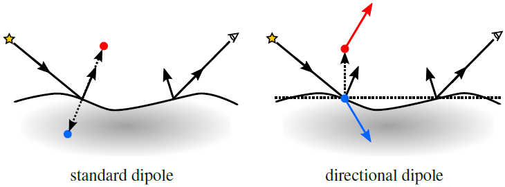
Our case study is analytical dipole models for simulating subsurface scattering of light. We compare the standard dipole and a new directional dipole (see the figure below).
|
| Figure. A standard dipole model uses two point sources to handle boundary conditions. The points are displaced along the normal at the point of incidence. The directional dipole model uses two directional sources that are displaced along the normal of a plane containing the points of incidence and emergence. |
The simulation consists of a bidirectional surface-scattering reflectance distribution function (BSSRDF) which depends on a rather large number of input parameters. The scattering material is described by the optical properties listed in the table in the example below. In addition, the BSSRDF depends on the surface points of incidence and emergence, the surface normals in these points, and the directions of incidence and emergence of the light. The reflectance returned by the BSSRDF is a scalar. The attribute data is thus scalar in the outset. The question is now how to visualize this function in a way that supports comparison of models.
Let us discuss the steps in the visualization pipeline. To import data, we implement the BSSRDF in the shading language (GLSL) part of a WebGL program. The point of incidence and the normal at the point of incidence are set to constants. Optical properties, the eye point, and the direction of incidence are uploaded as uniform variables, while the point of emergence and the normal at this point are uploaded as vertex attributes and interpolated across the surface triangles using varying variables. In this way, we support sampling of the BSSRDF in an unstructered grid. To perform data filtering, we choose to draw a 4 by 4 by 4 cube and let the point of incidence be the centre of the top face with a fixed normal along the $y$-axis. The direction of incidence is in the $xy$-plane with an angle of incidence specified by user input. We also enable user modification of the incident radiance, so that the user can scale the visualization result. Since it can be hard to compare reflectance values if they are visualized as grey scale pixel intensities, we perform data mapping using a logarithmic function. We consider the result of this to be the hue and obtain a false-colour visualization using hsv to rgb colour mapping. Finally, the data rendering happens through the WebGL rasterization pipeline.
The effect of subsurface scattering of light is translucency of the illuminated object. The translucency of an object is determined by the optical properties of its material. These parameters and the intensity of the incident illumination (incident radiance) can be set in the following table.
| Incident radiance $L_i$ | |
| Scattering coefficient $\sigma_s$: | |
| Absorption coefficient $\sigma_a$: | |
| Asymmetry parameter $g$: | |
| Index of refraction $\eta$: | |
Approximate single scattering is added to the standard dipole model.
Mouse control: orbit - left button, zoom - middle button, pan - right button.
Keyboard options: larger angle of incidence - [+], smaller angle of incidence - [-], toggle colour mapping on/off - [m].